Vol. 1, No. 4
The Housing Market Part 9. Plus, Stock Valuation Rundowns and a Deep Dive on My Best Idea.
Welcome to Valuabl - a fortnightly newsletter for value investors with in-depth research, stock valuation rundowns, and deep dives on my best ideas.
Useful links: Book | Course | Requests | Twitter | Guide
In Today’s Issue:
Housing Market: Part 9: A Long Term Look at Intrinsic Values (11 minutes)
Stock Valuation Rundowns (3 minutes)
Deep Dive on My Best Idea (13 minutes)
1/ Housing Market: Part 9: A Long Term Look at Intrinsic Values
I’m sure that long term readers of Valuabl are utterly fed up with my discussion of the housing market. No topic seems to elicit as much emotion from both sides of the table as this one does. And, despite my best efforts, I am consistently drawn back to this topic.
In Part 7 of this series, I wrote that:
“This post will, hopefully, conclude our discussion of the housing market.”
Then, in Part 8, I sought to address the counterpoint that population growth, combined with limited supply, would drive prices and values up forever.
However, the hardcore sceptics of my approach to valuing housing continue to say that I should stick to businesses because traditional valuation methodologies like Discounted Cash Flow analysis don’t apply to real estate.
Initially, I tried to dispel this by introducing the idea of aggregate ownership, but on its own, that argument still feels lacking. So, the question is, how has the traditional valuation methodology performed historically for housing? Has it been a reasonable estimate of intrinsic value, or am I delusional?
Before I tuck into that, let’s recap where we’ve been so far for newer readers.
Where We’ve Been
In Part 1, I established an enormous gap between the price and intrinsic value of the average house in the United Kingdom.
In Part 2, I demonstrated how the gap between value and price accounted for a roughly £83 trillion global bubble. I hypothesised about the three legs of the housing bubble stool (culture, financing, risk).
In Part 3, I illustrated how the modern housing market meets the S.E.C.’s criteria for a Ponzi scheme.
In Part 4, I explained that price discovery in the housing market is slow and that should the market turn, a slow ongoing Japan-style deleveraging was much more likely than a crash.
In Part 5, I disputed some of the most common objections to my analysis. I highlighted the link between the biased methodology banks measure mortgage risk and the self-perpetuating nature of monetary expansion.
In Part 6, I valued each of the housing markets in the OECD and highlighted the countries that were most at risk of housing bubbles.
In Part 7, I looked at long-run real house prices in the United States, introduced the concept of aggregate ownership, the Cantillon effect and its role in the bubble, and highlighted the Minsky cycle.
In Part 8, I addressed the counterpoint that limited supply and a growing population increases real prices. I looked at 710 years worth of house prices (US, UK, Amsterdam) and demonstrated no long-run relationship between real house prices and population. Moreover, I showed that real prices move with the credit cycle and that the rapid price appreciation of the last 25 years is abnormal.
The Valuation Methodology
My analysis assumes that the intrinsic value of real estate comes from the rent you could charge (or don’t charge to yourself). As a result, I value the housing market in aggregate (or on average) as a stable asset whose cash-flows (driven by rents) will grow in line with the economy forever.
The fundamental assumptions of this are:
Rents are revenue and cannot grow faster than the economy forever.
The economy will grow at the risk-free rate in perpetuity.
There is no growth reinvestment required, and maintenance reinvestment matches depreciation.
To see how this methodology performs over time, I have again relied on the brilliant work of Matthijs Korevaar, Marc Francke, and Piet Eichholtz of Maastricht University. They have created a long-term house price and rent index for the Amsterdam city centre from 1620 to 2019 (I added 2020 using the city averages). You’ll be familiar with this dataset as I used it in Part 8.
Long-Term Valuations and Prices
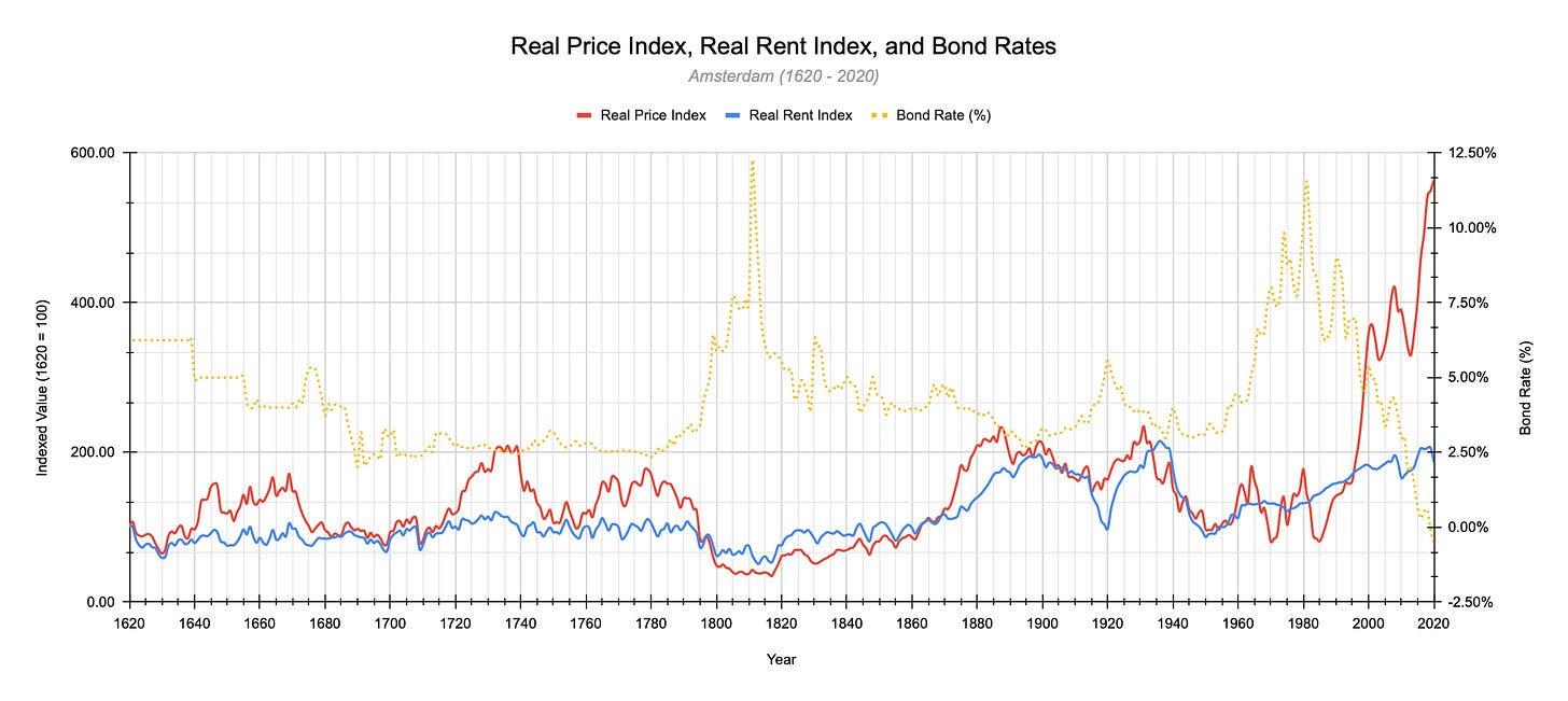
Below, I have plotted the real price index, the real rent index, and the government bond rate for Amsterdam and The Netherlands.

As I pointed out previously, if you bought a house in Amsterdam in 1619 and sold it in 1986, your real capital gain would have been zero. That is 370 years of holding for no capital gain in real terms. However, in the 35 years since, you would have realised a 559% real capital gain (!?). But, the question is, does the underlying intrinsic value justify this. Moreover, is that valuation methodology even applicable?
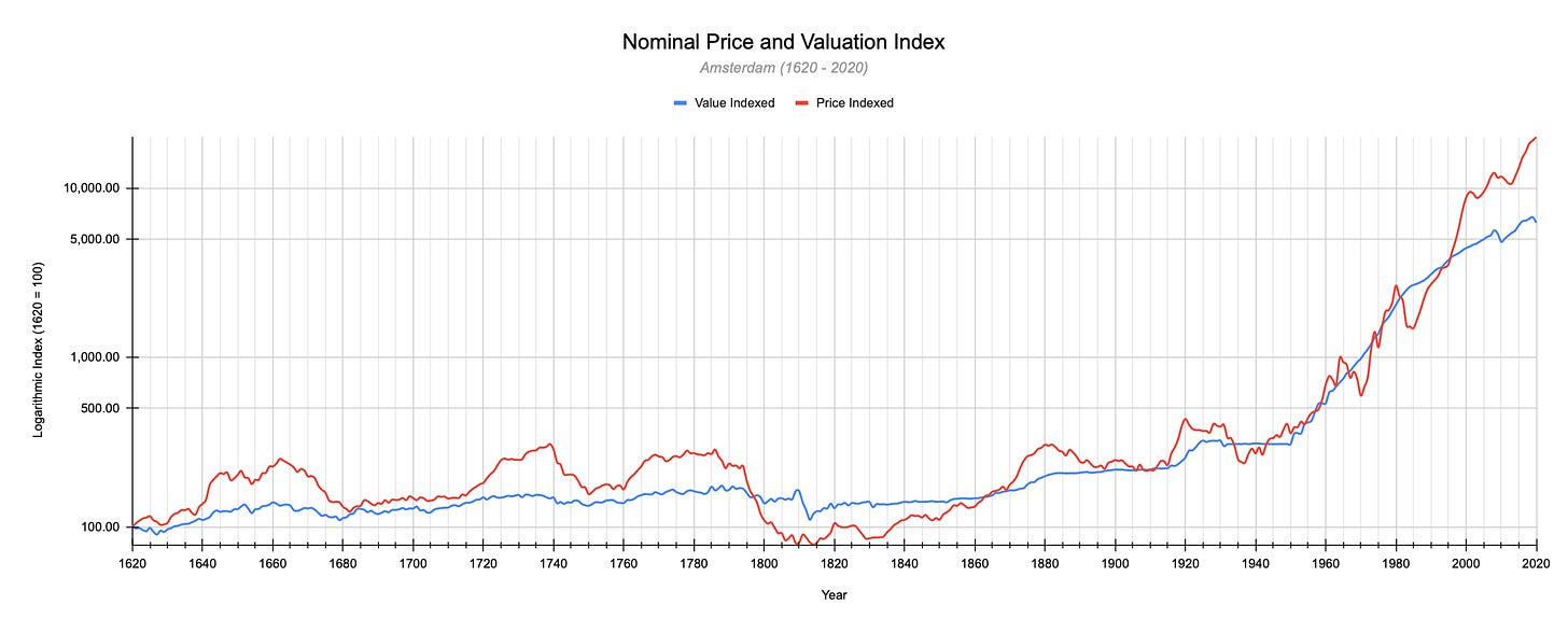
The following chart plots the nominal price and my intrinsic value index based on rents and bond rates. I have used a logarithmic scale.

The first thing we notice is that there seems to be a reasonably strong relationship between my estimate for the intrinsic value index and the price index. In fact, across all 400 years, there is a 0.94 correlation (p<0.01) between the two, and a chi-squared goodness-of-fit test on the two gives a p<0.01.
Going back to the original question:
… how has the traditional valuation methodology performed historically for housing? Has it been a reasonable estimate of intrinsic value, or am I delusional?
The answer is that it has been an excellent estimator of intrinsic value, but on average, and over time.
Now, we care about the difference between price and value and whether this suggests a bubble.
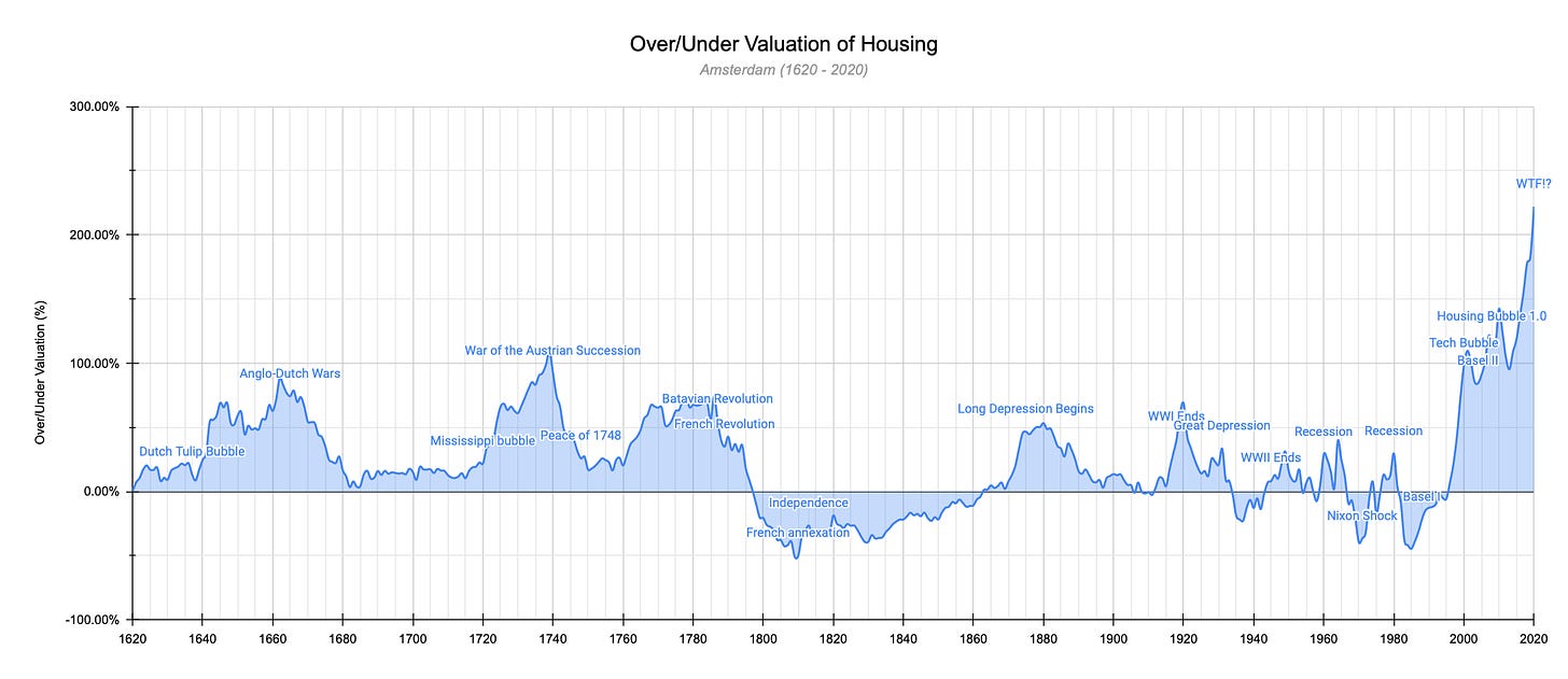
I have plotted the difference between the nominal price index and my intrinsic valuation index in the following chart. Moreover, I have overlaid significant historical, financial, and economic events.

Based on this, we will look briefly at eight different periods:
1620 - 1680: We can see that the exuberance and conditions that created the Tulip Mania (1634-1637) led to a housing bubble. The Dutch were the preeminent commercial superpower, and the Guilder effectively became the global reserve currency around 1640. House price continued to rise much faster than values, and by 1662 the difference was almost 89 per cent. However, increasing geopolitical tension and the English wanting to end Dutch domination of world trade instigated a series of wars between the two. The first of which started in 1652, the second in 1665, and the third in 1672. By 1682, house prices had declined back to their intrinsic level.
1680 - 1720: From 1680, the relative commercial power of the Dutch began to decline, and by 1720 they were no longer the preeminent global commercial superpower - the French were. During this period, the price of housing grew slowly and steadily in line with intrinsic values.
1720 - 1760: As the French were becoming the global superpower, Louis XIV had borrowed most of the gold in the country to build his palace (Versailles), fund war efforts, and pay for his lavish tastes. As I have outlined previously, following Louis XIV’s death, the Regent implemented a series of fractional-reserve-style, fiat monetary policies to pay back these debts that helped create the Mississippi bubble. Moreover, this led to such a rapid appreciation in house prices that the French began using the word ‘millionaire’ to describe their newfound wealth. French money flowed up and into Amsterdam, and the housing bubble peaked at 109 per cent over intrinsic value in 1738. The War of the Austrian Succession, which began in 1740, popped the bubble. By the time France had conquered most of the Austrian Netherlands in 1748, house prices in Amsterdam had roughly halved and were only 17 per cent overvalued. As part of the 1748 peace deal, France agreed to withdraw from the Austrian Netherlands and left it under the rule of the Habsburg Monarchy.
1760 - 1800: By 1780, the Dutch were in a deep economic crisis. The Fourth Anglo-Dutch War had taken its toll, housing was almost 70 per cent overvalued, and there was great social unrest and economic division. A sizeable political division between the ‘haves’ (wealthy landowning elite who supported William V) and the ‘have-nots’ led to the rise of the Patriots. They wanted to overthrow the current political system. Between 1783 and 1787, they took control of several regions, and by 1795, William had fled to England, and the Patriots had formed the Batavian Republic. By 1797, house prices in Amsterdam had again fallen to their intrinsic value.
1800 - 1860: By 1805, the Batavian Republic was under the control of Patriots who were sympathetic to the revolution that had taken place in France and wanted to side with Napoleon. In 1806, they formed the Kingdom of Holland, and Louis Napoleon became King. Following this, in 1810, the Kingdom of Holland was annexed into the First French Empire, and the price of housing in Amsterdam was roughly half of its intrinsic value. Then, in 1813, the Kingdom of Holland regained its independence from the French, and the British Pound became the global reserve currency. A prolonged period of economic and political stabilisation followed. By 1863, house prices in Amsterdam had recovered to their intrinsic value.
1860 - 1900: The Dutch economy continued to expand, and in 1870 the Bank of England accepted the role of ‘lender of last resort during a crisis. This new role coincided with a war between the French and British, which resulted in the Bank of England extending its financial power across Europe. In 1871, the Dutch formed a universal workers union and prioritised homeownership. But, a rapid expansion of the monetary supply drove house prices up. Between 1871 and 1875, prices rose by 47 per cent and were almost 50 per cent overvalued. However, the implementation of the international gold standard in 1875 curtailed the expansion of the money supply. Furthermore, the Second Industrial Revolution saw the proliferation of telegraph, railroad and utility networks and allowed an unprecedented movement of people. These two factors combined meant that house prices in Amsterdam declined until 1897, where they reached intrinsic value.
1900 - 1996: This period saw overvaluations peak during the First World War, the Second World War, and the recessions of the 60s and 80s. It’s fascinating to see how the housing cycle (short-term credit cycle) starts to come into force during this period, but valuations remain around intrinsic value. From 1900 to 1996, the average overvaluation using this approach was less than four per cent and is statistically insignificantly different from zero.
1996 - Now: Since 1996, prices have exploded compared to intrinsic values. First, they peaked during the Dot Com Tech Bubble before declining a little. They peaked again during the 2008 Housing Bubble before dropping a little. And, finally, in 2020, we hit 222 per cent overvaluation. The highest level ever.
Household Credit is The Key
In previous newsletters, I explained how monetary expansion through the credit cycle drives prices. But, let’s put some numbers on it and take a look at the relationship between household credit and real house prices.
To do this, I looked at two datasets from the Bank for International Settlements and analysed the relationship between their changes over time:
Total credit to households as a percentage of GDP.
Real residential property prices indexed.
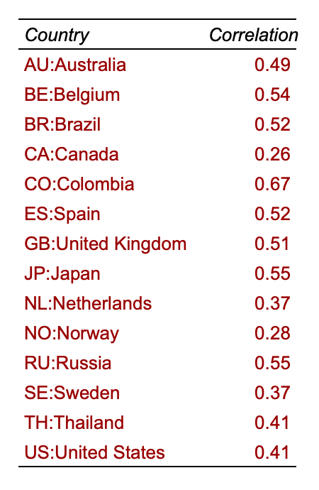
These datasets cover 41 counties across various lengths of time. Of the 41 countries in the dataset, 14 had statistically significant relationships between changes in the level of household credit (as a percentage of GDP) and real residential property prices. Of course, the results won’t surprise you; it’s the usual housing bubble suspects.

However, this dataset is not exhaustive, and many of the countries in the original 41 have too short datasets to observe anything meaningful.
The Lessons of History
So, what lessons can we draw from Amsterdam’s residential property bubbles of the past?
If we define the bubble as beginning when there is at least a 25 per cent overvaluation, then Amsterdam has had five bubbles (excluding the current one) going back to 1620.
For those five bubbles, the average time from the bubble beginning (reaching 25 per cent overvaluation) to reaching the peak was 15 years. The most extended buildup was 27 years for the 1759 - 1794 bubble.
If you bought around the peak, the average break-even time (on a nominal price basis) was 84 years. If you bought around 1739, it took 179 years to break even.
If you bought around the peak, your average annualised return for the next five years was -4.2 per cent, for the next ten years was -3.4 per cent, for the next 25 years was -2.1 per cent, and for the next 50 years was -1.1 per cent.

Moreover, what is the general predictive capacity of future returns from the level of over/undervaluation? In other words, do high levels of overvaluation predict negative future returns and do high levels of undervaluation indicate positive future returns.
There is a statistically significant negative relationship between the level of over/undervaluation and future returns, which means that high levels of overvaluation are a good predictor of future negative returns. And, in contrast, high levels of undervaluation are a good predictor of future positive returns.
The Future of Residential Real-Estate Prices
For Amsterdam, based on defining a bubble as starting when there is a 25 per cent overvaluation, the current bubble began in 1998 — this means we are 22 years into the bubble cycle. This is seven years more than the average and five years fewer than the most prolonged buildup (the bubble of 1759 to 1794). Moreover, the current bubble is dramatically larger than any previous bubbles, suggesting more pronounced negative future returns.
I first posted this research on Twitter. You can go there to follow me and get timely updates on my research.

2/ Stock Valuation Rundowns
Over the past fortnight, I valued:
Walmart, Inc. (NYSE: WMT)
The Coca-Cola Company (NYSE: KO)
Tyson Foods, Inc. (NYSE: TSN)
If you’re a subscriber, you can post your valuation requests here.
Walmart, Inc. (NYSE: WMT) - Valuation on November 11, 2021
Previous valuation: February 26, 2021
Walmart ($414 billion market cap) is a low-cost, American retailing behemoth. They are the world’s largest company by revenue ($566 million LTM) and are the dominant force in U.S. retailing (32 per cent of physical and 9 per cent online). Both online and offline retail markets will grow at a modest clip (between 4.8 and 6.8 per cent CAGRs) across Walmart’s segments. Still, they will continue slowly losing market share (currently 4.6 per cent of the global market) to more focused businesses with differentiated USPs. The company’s Every Day Lowest Price promise will limit any margin expansion (6.1 per cent is the highest level since ‘92); however, investments in automation (warehousing and self-driving trucks etc.) will help offset cost inflation. The company has an attractive cost structure (0.27x operating leverage), a robust credit rating (Aa2/AA) and a modest amount of debt (13 per cent market EV). However, they do face some additional country risks from their developing markets operations.


